Connecting LeanXcale with R

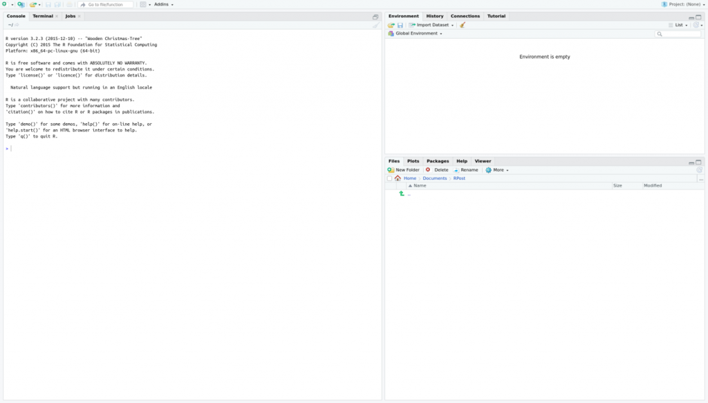
Hi! In this post, I demonstrate how to connect an R application to a LeanXcale database with the LeanXcale JDBC driver.

As you may know, R is a language and environment for statistical computing and graphics. According to its website, R provides a wide variety of statistical (e.g., linear and nonlinear modelling, classical statistical tests, time-series analysis, classification, and clustering) and graphical techniques, and is highly extensible. R is widely used for data science thanks to its nearly 12,000 libraries that enable it to perform any statistical analysis on data. This broad applicability makes it very interesting to be able to integrate R capabilities with the strengths of LeanXcale.

This post can be your building block for developing an R application with a LeanXcale database by following the basic steps to set up an environment and use the JDBC LeanXcale driver through the RJDBC R library. All required files and code samples are available in our GitLab repository.

Prerequisites

To execute the steps presented in this post, you need to meet several prerequisites. First, you must configure an environment in which you can work with R. I next guide you through the steps to install R and RStudio in a Linux environment.

I install the latest R version, which is 4.0.2, at the time of writing. To do so, you should first add the correct repository into our /etc/apt/sources.list by adding at the end of the file the following line, according to the official documentation:

NOTE: I have Ubuntu 16.04 Xenial installed, so if you have a different version of Ubuntu, then please select the appropriate entry.

Next, add the repository server key in your system:

sudo apt-key adv --keyserver keyserver.ubuntu.com --recv-keys E298A3A825C0D65DFD57CBB651716619E084DAB9

Finally, update your system package index with the following command entered in a terminal:

sudo apt update

To install the base R, enter the command:

sudo apt -y install r-base

Once R is installed, RStudio is next installed by clicking through to https://rstudio.com/products/rstudio/download/#download and downloading the version desired for your platform.

After the download is complete, install it by entering the command:

sudo dpkg -i <RStudio.deb data-preserve-html-node="true">

NOTE: In my case, I manually installed some dependencies by entering the following commands:

sudo apt install libclang-dev 
sudo apt -f install

After these steps are complete, you will have installed R and the IDE, RStudio, ready to use.

Downloading the JDBC driver

LIBRARIES REQUIRED

To use the LeanXcale JDBC driver, the R package RJDBC must be installed into your environment. To install this package from within RStudio, you execute through the R Console:

install.packages("RJDBC", dep=TRUE)

If you have not configured rJava, then you may need to run, prior to the command above, the following command in a Linux terminal:

sudo R CMD javareconf

If the installation completed without error, then you can check for the installed packages under the packages tab in the User Library: rJava and RJDBC.

LEANXCALE JDBC DOWNLOAD

To download the Leanxcale JDBC driver, you can click through to the drivers page on the LeanXcale website and download the JDBC jar with its dependencies at https://docs.leanxcale.com/leanxcale/current/1.4/index.html.

I use an on-premise LeanXcale installation, and if you want to use LeanXcale to follow along with this post, then you can request a free trial.

Development

Because the purpose of this post is to show you how to interact with LeanXcale from R, I next import some data and perform analytical queries using the JDBC driver. The dataset I use here is the well-known Boston Housing dataset.

DATASET AND TABLE CREATION

This dataset was collected in 1978 and consists of aggregated data concerning houses in different suburbs of Boston, with a total of 506 cases and 14 columns. According to the Boston Housing Dataset website, we interpret each of the 14 variables as follows:

CRIM – per capita crime rate by town.
ZN – proportion of residential land zoned for lots over 25,000 sq. ft.
INDUS – proportion of non-retail business acres per town.
CHAS – Charles River dummy variable (1 if tract bounds river; 0 otherwise).
NOX – nitric oxides concentration (parts per 10 million).
RM – average number of rooms per dwelling.
AGE – proportion of owner-occupied units built prior to 1940.
DIS – weighted distances to five Boston employment centers.
RAD – index of accessibility to radial highways.
TAX – full-value property-tax rate per $10,000.
PTRATIO – pupil-teacher ratio by town.
B – 1000(Bk – 0.63)^2 where Bk is the proportion of blacks by town.
LSTAT – % lower status of the population.
MEDV – median value of owner-occupied homes in $1000’s.

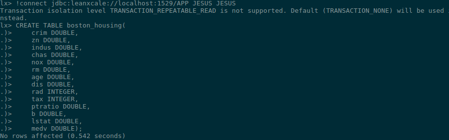
To reflect this data in our database, we recreate the schema formed for this example in a single table, which I call boston_housing. In the provided project code, you can find the SQL create script. To create the table, I use LeanXcale’s SQL client provided with the client package.

DATABASE CONNECTION

After you have the LeanXcale database prepared with the table created, you can start using the JDBC driver from within your R program. In this example, you need to adapt the connection URL to your specific case, specifying the address and port where your LeanXcale instance is running, along with the database, user, and password you use to connect. Also, you need to specify the path to your JDBC driver jar file you downloaded in the step above.

library(DBI)
library(rJava)
library(RJDBC)
drv <- RJDBC::JDBC("com.leanxcale.client.Driver",
classPath="/home/jesus/Documents/RPost/qe-driver-1.5.0-jar-with-dependencies.jar")
conn <- dbConnect(drv, "jdbc:leanxcale://localhost:1522/APP",
                  "JESUS", "JESUS")

LOADING PHASE

Now, I demonstrate how to perform insertions into LeanXcale using JDBC. If you read the CSV file and save it in memory using a dataframe, then you can directly call the dbSendUpdate on the connection previously created with the insert SQL and the dataframe that contains the data. This call handles executing the inserts with prepared statements and parameterized queries.

setwd("/home/jesus/Documents/RPost")
df <- read.csv(file = "BostonHousing.csv")

sql = "INSERT INTO JESUS.boston_housing values 
 (?, ?, ?, ?, ?, ?, ?, ?, ?, ?, ?, ?, ?, ?)"

rs <- dbSendUpdate(
    conn,
    sql, list=df)

ANALYTICAL QUERIES

Once the data is loaded into the table, I perform several basic analytical queries to show the functionality and how easily we can construct more complex queries in RJDBC.

To stay within the scope of this post, I simply execute a full scan and basic aggregations, such as max, min, and mean over the target column, the house pricing value MEDV.

In JDBC, executing the SQL query using a statement is enough to retrieve the desired data from the resultset. To execute the SQL query, use the dbSendQuery method that returns the resultset. Although, to get the result from the resultset, you must first call dbFetch.

sql_analytics = "SELECT MIN(MEDV) AS MIN_PRICE, MAX(MEDV) AS MAX_PRICE, AVG(MEDV)
AS MEAN_PRICE FROM JESUS.boston_housing"
rs <- dbSendQuery(conn, sql_analytics)
result <- dbFetch(rs)
View(result)
dbClearResult(rs)

Conclusion

Now that you have read this post and, hopefully, completed all the steps, you know how to integrate an R application with a LeanXcale database using the LeanXcale JDBC driver. Also, you learned how to insert data using RJDBC updates, and you performed several SQL example queries to prepare you to extend to more complex queries for your applications.

Happy coding!