To improve its behavior as a transactional and analytical processing (HTAP) database, LeanXcale provides a new feature for supporting online aggregations using a specifically created type for it. Find here an application of online aggregations in LeanXcale for group-by queries and learn how it works.

Abstract

Imagine we want to build a dashboard to analyze the users that are visiting a website every second. If we don’t want to implement lambda architecture and we only want to use a database, we would have to periodically execute count-group-by queries at the time of the insertion with the condition of not losing performance, either in queries or in the insertion. As there are usually many more insertions than reads, caching reads in memory is possible, but this doesn’t sound too good. What if we had a database that pre-calculated counts at the time of the insertion, with absolute fresh data and without affecting the insertion? This would serve the aggregate in real-time. SPOILER: LeanXcale can do it!

To improve its behavior as a transactional and analytical processing (HTAP) database, LeanXcale provides a new feature for supporting online aggregations using a specifically created type for it. LeanXcale’s delta type support for online aggregation means that the result of an aggregation query, such as a count-group-by clause, is pre-calculated at the time of insertion. This way, getting the aggregate for a value requires simply reading a row from the relevant aggregate table, which is already pre-calculated, instead of doing a scan to find the right row and calculate the aggregation. This means aggregations in real-time.

Introduction

Hybrid transaction/analytical processing (HTAP) is a term created by Gartner to describe the situation in which OLTP and OLAP capabilities operate on the same database instance. It is then possible to execute operational transactions and load operations for analysis over the same database instance in real-time, while not affecting operational transactions by analytical issues, as shown in the image:

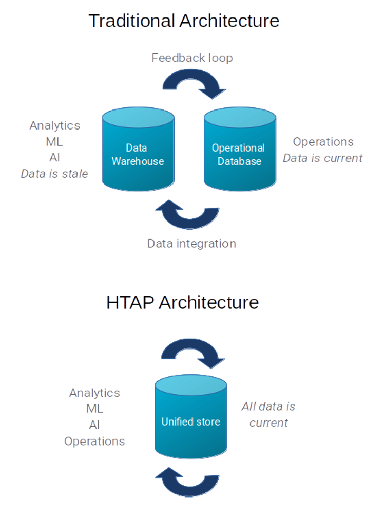
This way, HTAP architecture can handle analytical queries and processes over ever-fresh data, always ensuring that operational systems are not affected by analytical processes. There is no need to execute, for example, ETLs to extract data once or twice a day from the operational databases to the data warehouse databases. HTAP architecture eliminates the delay and some of the problems commonly associated with ETLs.

A common approach to solving these issues when no HTAP database is available is to implement a lambda architecture, in which batch processing, real-time processing, and query executions are done in separate layers and by different technology. Examples of such technology include Hadoop for batch processing, Spark for real-time processing, and Druid for query execution layer. If we have real-time complex processes, the lambda architecture is the best approach. But if we only want to calculate aggregates in real-time, this architecture might be like using a sledgehammer to crack a nut.

If we don’t want to implement a complex architecture simply to calculate aggregates in real-time, to help analysts understand and evaluate data it is common to execute many group-by queries on the sets of the columns of interest. Considering the usual volume of data in databases prepared for analytical operations, and also the number of columns often contained in tables, executing a large number of group-by queries can make it too expensive to use HTAP architecture. If we can have fresh data at any time but queries are too expensive to execute, we must deal with delays that significantly impoverish the capacity of an HTAP database.

LeanXcale is specially designed for supporting HTAP architecture: operational processes are not affected when executing analytics queries. Besides, it supports online aggregation, which means that aggregation computing, such as a group-by clause or a sum, is pre-calculated at the time of insertion. This way, getting the aggregate requires simply reading a row from the relevant aggregate table, which is already pre-calculated, instead of doing a scan to find the right rows and execute the aggregation (which requires much more computation at the time of the query).

In this post, we are going to illustrate how to configure an online aggregation with LeanXcale over a group-by query. To demonstrate its power, we will perform a comparison of the architecture and the response time for these kinds of queries between LeanXcale and PostreSQL.

OK, But… What is this for?

The short answer: it’s for calculating aggregates of any kind over a database without executing a heavy group-by query and without losing performance on an insertion. As this answer is a little boring, let’s imagine we want to build a monitorization application similar to the Google Analytics dashboard.

In general terms, when implementing these kinds of applications, it is necessary to consider two important things: the insertion performance and the query execution performance. Usually, when storing web access data, the number of insertions is going to be much higher than the number of reads, so it seems reasonable to prioritize insertion performance rather than reading performance.

This hypothetical application would report lots of things, such as the number of users visiting the web page. This used to be done with aggregations over users’ cookie IDs, and sometimes, with high volumes of data, these aggregation queries are too slow, and even worse, they may block insertions. Thus, we are losing currently inserted data; if there’s a high volume of insertions, reported data are not going to be real and fresh enough for our purposes.

To illustrate this, we have generated some controlled data to simulate the insertion of thousands of cookies per second. As an example, these could be possible rows:

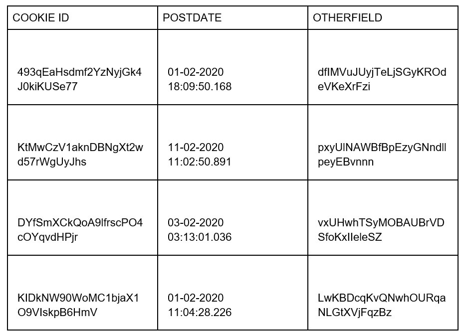
The cookie ID and the request postdate will be the primary key to our table. “Otherfield” is just a random-generated String. In real situations there will be other fields, for example, user’s session, browser, request URL, etc.

Let’s combine LeanXcale’s capacity of insertion and delta types for the purpose of monitoring cookies and see how it works!

Architecture and components

We need:

• A LeanXcale database instance. You can find it here.
• A PostgreSQL database instance. You can find it here.
• A program that simulates data insertion and executes queries periodically. You can find it here.
• A SQL client, we recommend SQuirreL. You can take a look at our install and setup instructions.

LEANXCALE AND DELTA TABLES

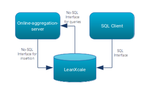
The LX global architecture consists of a loader and query executor program, a LX instance, and a SQL client. It uses different threads to insert and to execute queries. Of course, we can benefit from LeanXcale’s versatility, in which we can use either a No-SQL or a SQL interface. This means that, although in this example we are going to use our No-SQL interface for both insertion and query execution, we are always going to have the possibility of executing SQL queries. This makes it possible to query the aggregates using whatever BI tool we desire to use.

About the data model, we will create a table to store the cookie information and two additional tables to store the delta aggregates that will be pre-calculated at the time of the insertion.

POSTGRESQL AND ITS APPROACHES

About PostgreSQL, as there is no No-SQL interface, we will insert and query using JDBC from the server. Besides, about the data model, we have two direct options to implement the solution for our case.

• The first approach is to try to calculate the aggregation at the time of the insertion, which is the same idea LeanXcale works with. Unfortunately, PostgreSQL does not have something similar to LeanXcale’s delta type, and we have to create some trigger structure to calculate the aggregate and some other trigger structure for keeping data consistent in cases of row deletion. The bad news here is that the insertion time is going to be affected by the trigger’s execution. The good news is that the read time is going to be faster. There is also horrible bad news with this approach, and that is the possibility of causing a deadlock in Postgres between the insertion of a new row and a trigger execution on the last inserted row if we don’t commit after inserting each row. This is the expected behavior in a trigger, so it does not seem possible to avoid it. For our comparison, we are only going to insert from a data source, which is a single thread loading the CSV data row by row.
• The second approach is to execute the aggregation queries by using a common group-by query. The good news about this approach is that the insertion time gets less affected. The bad news is the performance is worse when executing count-group-by queries over high volumes of data.

Although the right approach for our hypothetical analytics application would be to prioritize insertion performance over read performance, let’s try both approaches. We can define two scenarios:

• Scenario 1: LX with delta tables versus PostgreSQL with trigger structure. In this scenario, in PostgreSQL, we prioritize data reads over insertion performance.
• Scenario 2: LX with delta tables versus PostgreSQL executing classic group-by queries. In this scenario, in PostgreSQL, we prioritize insertion performance over reading performance.

For scenario 1, in PostgreSQL, we need:

• A trigger after inserts for every aggregate we want to serve. This trigger will analyze the new row, look for it per primary key on a specifically created table, and add 1 to the value.
• A trigger after a delete for every aggregate we want to store, to keep data consistency. This new trigger will analyze the new row, look for it per primary key on a specifically created table, and subtract 1 from the value.

For this demo, we can consider that there will be no deletions, and thus the second trigger will not be created; we will work only with the first one. Please note that we are going to need a trigger and a specific table for each aggregation to calculate.

For scenario 2, in PostgreSQL, we need nothing but the database and the structure of the main table.

HOW TO CREATE AND OPERATE A DELTA TABLE IN LEANXCALE

Let’s go! The data inserter program is, again, like data inserters in other posts, and is built with Java and Spring Boot. It will respond to three kinds of requests:

• Run: to start the insertion.
• Clean: to clear the database.
• Query: to start the periodic query executor.

This program is implemented using the usual code design with the controller, service, and some implementations to create the database structure, to read and insert the CSV files, and to execute queries. You can find source code here. We are using CSVs for insertion because we have found this to be the fastest way to insert the same data in both databases, as we have the data previously generated.

You can download the Java KiVi Direct API (No-SQL library for LeanXcale) from our website and define the dependency as follows:

mvn install:install-file -Dfile=kivi-api-1.4-direct-client.jar -
DgroupId=com.leanxcale -DartifactId=kivi-api -Dversion=1.4 -Dpackaging=jar

<dependency>
   <groupId>com.leanxcale</groupId>
   <artifactId>kivi-api</artifactId>
   <version>1.4</version>
</dependency>

First, we have to create the main table and the aggregate tables. Let’s create a very simple table, with an alphanumeric ID and a timestamp, both acting as composite primary keys. The idea is to simulate the insertion of a cookie and its access timestamp; cookie IDs are not unique, but the pair formed by the cookie and its access timestamp it is. We are also going to create a field called “otherfield”; in real use cases, the desired fields may be added.

private static final String TABLE_NAME = "INFO"

(…)

Settings settings = new Settings();
     settings.setUrl(URL);
     settings.setUser(user);
     settings.setDatabase(databaseName)
     settings.transactional();
        
try (Session session = SessionFactory.newSession(settings)) { // New session
// Table creation: 
if (session.database().tableExists(TABLE_NAME)) {
       // Primary key fields
        List<Field> keyFields = Arrays
                     .asList(new Field[]{new Field("id", Type.STRING),
                             new Field("postdate", Type.TIMESTAMP)});
             // Rest of fields
             List<Field> fields = Arrays
                     .asList(new Field[]{
                                  new Field("otherfield", Type.STRING)
                                  });
             // Table creation
             session.database().createTable(TABLE_NAME, keyFields, fields);
       }
}

The above code is equivalent to the SQL code:

create table INFO (
  ID VARCHAR,
  POSTDATE TIMESTAMP,
  OTHERFIELD  VARCHAR,
  CONSTRAINT PK_INFO PRIMARY KEY (ID, POSTDATE)
);

Once created, let’s think of the group-by queries we want to execute.

It’s common, for example, to try to know how many different users have visited our page and how many times; to do this, we have to execute a SQL query such as:

select id, count(id) from info  group by id;

But when we are handling millions of rows, these kinds of queries may be very heavy and slow. The same thing would happen if, for example, we wanted to know how many visits per day our page has had. This new datum could be extracted with a query like:

select FLOOR(POSTDATE to DAY) as fecha, count(*) AS total FROM info group by 
FLOOR(POSTDATE to DAY);

That would have the same problem as the previous one.

So, what if we pre-calculate the aggregate and get it with the same cost of accessing a row by PK?

As mentioned above, LeanXcale offers a special data type called “delta” to pre-calculate the aggregate value. Let’s create the aggregate tables for pre-calculation. We are going to create one table per aggregate we need. In this case, we need two tables: one for ID count and another one for date count.

The field from which we are going to aggregate must be the aggregate table PK, and the aggregator must be defined as delta in the field creation.

private static final String ID_COUNT_DELTA_TABLE_NAME = "INFO_ID_DELTA";
private static final String DATE_COUNT_DELTA_TABLE_NAME = "INFO_DATE_DELTA";

(…)

Settings settings = new Settings();
     settings.setUrl(URL);
     settings.setUser(user);
     settings.setDatabase(databaseName)
     settings.transactional();

try (Session session = SessionFactory.newSession(settings)) { // New session

// Aggregation table creation:
if (!session.database().tableExists(ID_COUNT_DELTA_TABLE_NAME)) {
   List<Field> keyFields = Arrays
           .asList(new Field[]{new Field("id", Type.STRING)});
   List<Field> fields = Arrays
           .asList(new Field[]{
                   new Field("count", Type.LONG, DeltaType.ADD)});
   session.database().createTable(
           ID_COUNT_DELTA_TABLE_NAME, keyFields, fields);
}
// Aggregation table creation:
if (!session.database().tableExists(DATE_COUNT_DELTA_TABLE_NAME)) {
   List<Field> keyFields = Arrays
           .asList(new Field[]{new Field("postdate", Type.DATE)});
   List<Field> fields = Arrays
           .asList(new Field[]{
                   new Field("count", Type.LONG, DeltaType.ADD)});
   session.database().createTable(
          DATE_COUNT_DELTA_TABLE_NAME, keyFields, fields);
}
}

We have defined two tables, one per aggregate:

• The first table, INFO_ID_delta, corresponds to query select id, count(id) from info group by id;. Since we want to group it by ID, the ID is going to be the PK of this delta table. The aggregate will be the count, and we will add 1 to the precalculated aggregate (please note the delta field is declared as DeltaType.ADD).
• Similarly, the second table, INFO_DATE_delta, corresponds to query select FLOOR(POSTDATE to DAY) as fecha, count(FLOOR(POSTDATE to DAY)) AS total FROM info group by FLOOR(POSTDATE to DAY); the table PK is going to be the postdate field, and the aggregate will again be the count.

Now that we have created the table infrastructure, let’s do the insertion. While inserting into the main table INFO, we also have to do the insert on the aggregate tables.

try (Session session = SessionFactory.newSession(settings)) { // New session
     session.beginTransaction();
     Table infoTable = session.database().getTable(TABLE_NAME);
     Table infoIdTable = session.database().getTable(ID_COUNT_DELTA_TABLE_NAME);
     Table infoPostdateTable =   
           session.database().getTable(DATE_COUNT_DELTA_TABLE_NAME);

     // Insert into info table
     Tuple tuple = infoTable.createTuple();
     tuple.putString("id", id);
     SimpleDateFormat dateFormat = new SimpleDateFormat(
                                              "dd-MM-yyyy HH:mm:ss.SSS");
     Date date = dateFormat.parse(postdateString);
     tuple.putTimestamp("postdate", new Timestamp(date.getTime()));
     tuple.putString("otherfield", otherfield);
     infoTable.insert(tuple);

     // Insert into info_id_delta
     Tuple tupleIdDelta = infoIdTable.createTuple();
     tupleIdDelta.putString("id", id);
     tupleIdDelta.putLong("count", 1L); // We add 1 to our DeltaType.ADD field
     infoIdTable.upsert(tuple);

     // Insert into info_date_delta
     Tuple tupleDateDelta = infoPostdateTable.createTuple();
     tupleDateDelta.putDate("postdate", new java.sql.Date(date.getTime()));
     tupleDateDelta.putLong("count", 1L);
     infoPostdateTable.upsert(tupleDateDelta); // We add 1 to our DeltaType.ADD                         
                                                  field

     session.commit();
}

One might think the delta mechanism is similar in a classic database for implementing a trigger. But with a classic trigger we must:

1. Define an after insert trigger in the INFO table.
2. In the trigger code, we must look for the appropriate row in the delta tables and get the aggregate value.
3. Calculate the new aggregate value adding 1.
4. Write the new aggregate value.

In this scenario, the INFO table row remains locked from steps 1 to 4, and the delta table row remains locked from steps 2 to 4. Besides, it’s necessary to do a lookup on the aggregate tables, which will result in a significant performance loss at insertion time. With LeanXcale’s delta mechanism, there are no locks. First, this is because no code needs to be executed from the trigger, and second, the aggregate value is consolidated on the first read from the delta tables, instead of adding 1 on each insert.

About the periodic query execution, we are going to use the NoSQL interface provided by LeanXcale:

private Session session = null;

private Table infoTable;
private Table infoIdTable;
private Table infoPostdateTable;

private int executions = 0;

Settings settings = new Settings();
     settings.setUrl(url);
     settings.setUser(user);
     settings.setDatabase(databaseName)
settings.transactional();
settings.deferSessionFactoryClose(10000);

try{
   session= SessionFactory.newSession(settings);
   infoTable = session.database().getTable(Constants.TABLE_NAME);
   infoIdTable = session.database().getTable(Constants.ID_COUNT_DELTA_TABLE_NAME);
   infoPostdateTable = session.database().getTable(Constants.DATE_COUNT_DELTA_TABLE_NAME);

   while (executions < 1000) {
       log.info("-----------------------------------------------------------------------------------------------------------");
       log.info("LX: Querying info table for number of rows...");
       session.beginTransaction();
       // Build TupleIterable, execute find with count aggregation and iterate 
       // over the result (select count(*) from info) 
       TupleIterable res = infoTable.find().aggregate(Collections.emptyList(), Aggregations.count("numRows"));
       res.forEach(tuple -> log.info("Rows: " + tuple.getLong("numRows")));
       log.info("LX Querying info table done!");


       log.info("-----------------------------------------------------------------------------------------------------------");
       log.info("LX: Querying id delta table...");
       long t1 = System.currentTimeMillis();
       // select * from info_id_delta
       TupleIterable res2 = infoIdTable.find();
       res2.forEach(tuple -> log.info("Id: " + tuple.getString("id") + " Count: " + tuple.getLong("count")));
       long t2 = System.currentTimeMillis();
       log.info("LX Query time: {} ms", t2 - t1);
       log.info("LX Querying id delta table done!");

       log.info("-----------------------------------------------------------------------------------------------------------");
       log.info("LX: Querying postdate delta table...");
       long t3 = System.currentTimeMillis();
       // select * from info_date_delta
       TupleIterable res3 = infoPostdateTable.find();
       res3.forEach(tuple -> log.info("Date: " + tuple.getDate("postdate") + " Count: " + tuple.getLong("count")));
       session.commit();
       long t4 = System.currentTimeMillis();
       log.info("LX Query time: {} ms", t4 - t3);
       log.info("LX Querying id delta table done!");

       executions++;
       Thread.sleep(5000);
   }
}
finally {
   if (session == null) {
       session.close();
   }
}

APPROACH WITH TRIGGERS IN POSTGRESQL

As we are doing the comparison against PostgreSQL, we are going to create scenario 1 with some triggers. These are the SQL statements to create this scenario in PostgreSQL:

Create tables:

CREATE TABLE INFO (ID VARCHAR NOT NULL, 
              POSTDATE TIMESTAMP(3) NOT NULL, 
              OTHERFIELD VARCHAR, 
              PRIMARY KEY(ID, POSTDATE));

CREATE TABLE INFO_ID (ID  VARCHAR  NOT NULL,
                      AGGREGATOR INTEGER NOT NULL, 
                      PRIMARY KEY(ID));

CREATE TABLE INFO_POSTDATE (POSTDATE TIMESTAMP NOT NULL,
                            AGGREGATOR INTEGER NOT NULL, 
                            PRIMARY KEY(POSTDATE))

Create trigger functions:

CREATE OR REPLACE FUNCTION public.agg_id() RETURNS trigger LANGUAGE plpgsql AS $function$ 
 DECLARE  
  ident VARCHAR; 
  aggreg INT; 
 BEGIN 
  SELECT T.id, T.aggregator INTO ident, aggreg FROM INFO_ID T WHERE T.id = NEW.ID;
  IF IDENT <> '' THEN UPDATE INFO_ID SET aggregator = aggreg+1 WHERE id = ident; 
  ELSE INSERT INTO INFO_ID (id, aggregator) VALUES (NEW.ID, 1); 
  END IF;
  return null;
END;
$function$;

CREATE OR REPLACE FUNCTION agg_postdate() RETURNS TRIGGER LANGUAGE plpgsql AS $function$
 DECLARE  
  postdat TIMESTAMP; 
  aggreg INT; 
 BEGIN 
  SELECT T.postdate, T.aggregator INTO postdat, aggreg FROM INFO_POSTDATE T WHERE
  DATE_TRUNC('day',T.postdate) = DATE_TRUNC('day',NEW.POSTDATE);
  IF postdat is NOT NULL THEN UPDATE INFO_POSTDATE SET aggregator = aggreg+1 WHERE
  DATE_TRUNC('day',postdate) = postdat; 
  ELSE INSERT INTO INFO_POSTDATE (postdate, aggregator) VALUES
  (DATE_TRUNC('day',NEW.POSTDATE), 1); 
  END IF;
 return null;
END
$function$;

And create triggers:

CREATE TRIGGER TRIGGER_AGG_ID 
 AFTER INSERT ON INFO 
 FOR EACH ROW EXECUTE FUNCTION agg_id(); 

CREATE TRIGGER TRIGGER_AGG_POSTDATE 
 AFTER INSERT ON INFO 
 FOR EACH ROW EXECUTE FUNCTION agg_postdate();

Execution comparison

Let’s compare execution times. To insert, let’s use our inserter program mentioned above. The fastest way we have found to load the same data in both databases is to generate some CSV files and load them with a separate java thread for each one, and then insert exactly the same data in both databases.

As a brief explanation of the loader program, if you navigate over the code, the key classes are:

• com.leanxcale.service.creator.impl.LXMetadataCreatorImpl: Responsible for the creation of all database structures in LeanXcale. To modify it or create another implementation, it is only necessary to make the new class implement the com.leanxcale.service.creator.MetadataCreator interface, implement the required methods and inject the new implementation modifying the metadataCreatorFactory.properties file.
• com.leanxcale.service.creator.impl.PGMetadataCreatorImpl: Responsible for the creation of all database structures in PostgreSQL. It can be altered the same way as the previous class because both implement the same interface.
• com.leanxcale.service.loader.impl.LXCSVDataLoaderImpl: Responsible for reading the CSV files and inserting their rows into LeanXcale. Similar to the previous classes, to modify it or create another implementation, it is only necessary to make the new class implement the com.leanxcale.service.loader.DataLoader interface, implement the required methods and inject the new implementation modifying the dataLoaderFactory.properties file.
• com.leanxcale.service.loader.impl.PGCSVDataLoaderImpl: Responsible for reading the CSV files and inserting their rows into PostgreSQL. It can be altered the same way as the previous class because both implement the same interface.
• com.leanxcale.service.executor.impl.LXQueryExecutorImpl: Responsible for executing periodical queries over LeanXcale. Similar to the previous classes, to modify it or create another implementation, it is only necessary to make the new class implement the com.leanxcale.service.executor.QueryExecutor interface, implement the required methods, and inject the new implementation, modifying the queryExecutorFactory.properties file.
• com.leanxcale.service.executor.impl.PGQueryTriggerExecutorImpl: Responsible for executing periodical queries over PostgreSQL over the trigger structure. It can be altered the same way as the previous class because both implement the same interface.
• com.leanxcale.service.executor.impl.PGQueryCountExecutorImpl: Responsible for executing periodical queries over PostgreSQL over the structure for querying with the count. It can be altered the same way as the previous classes because all three implement the same interface.

You can download the inserter program code here and modify the onlineagg.properties file to set LeanXcales’ and PostgreSQLs’ host, database name, and credentials. It is also necessary to modify the csvList.properties file to indicate which CSV to load; the loader will load the specified CSV files on both databases.

Then, as it is a Spring Boot program, the only thing we must do is as follows, from the root folder of the project:

mvn spring-boot:run

This will start a server on port 8080 listening to run and clean requests.

You can also build a jar and execute it:

mvn clean package
java -jar online-aggregation-server-0.0.1-SNAPSHOT.jar

Now, you can use your favorite http client to make a request to http://spring-boot-server-ip:8080/OnlineAgg/run to start inserting. Please wait for the first CSV to be completely loaded in both databases.

To restart the database structure and drop all tables, use the request from http://spring-boot-server-ip:8080/OnlineAgg/clean and then call run again.

To start the periodic query executor, use the request from http://spring-boot-server-ip:8080/OnlineAgg/query.

You can download the complete set of results here.

SCENARIO 1: LX with delta tables versus PostgreSQL with trigger structure

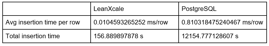
INSERTION TIME

With the table structures defined above, let’s compare the insertion times. We have logged the insertion time to two files doing nothing other than adding some System.currentTimeMillis() to the LeanXcale and PostgreSQL data loader classes. The files resulting of the load of the CSVs can be seen here.

In this scenario, we obtain a total insertion time gain of 98.95%, with LeanXcale over PostgreSQL, and a row average insertion time gain of 98.95%, again with LeanXcale over PostgreSQL. This means that LeanXcale stores 15 million rows in 2.65 minutes, whereas Postgres stores the same quantity of data in 4.21 hours. This approach with triggers does not seem to have the best performance in terms of insertions.

QUERY EXECUTION

First, let’s ensure that LeanXcale and PostgreSQL return the same values for the aggregate.

select * from info_id_delta; --LeanXcale
select * from info_id; --Postgres

The results:

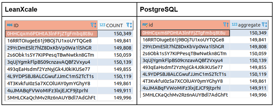
OK, the results are the same for both databases.

Now, let’s analyze the response times from the logs. These are the first results registered for the first aggregator, based on our application’s cookie ID. As there is a high number of queries periodically executed, let’s analyze the last 10 queries.

Last 10 queries aggregating per ID:

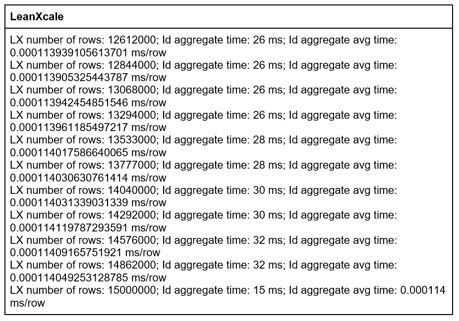
Although we can see that the aggregate time in LeanXcale in absolute value rounds is 28 ms and the aggregate time in Postgres rounds is 2 ms, which means a significative difference, if we have a look at the aggregate average time value, we can see LeanXcale aggregating in 0.00011 ms/row, while Postgres aggregates in 0.00033 ms/row. This is because, as LeanXcale inserts much faster, the aggregate that it must calculate aggregates more rows than the aggregates PostgreSQL must calculate. That means a gain of 66% in an average aggregation time with LeanXcale over PostgreSQL. Besides, if we have a look at the relative gain considering the insertion time, we have Postgres loading 15 million rows in 4.21 hours and aggregating with an average time of about 0.00033 ms/row. However, we have LeanXcale loading 15 million rows in 2.65 minutes and aggregating with an average time of around 0.00011 ms/row.

About the date aggregator, let’s ensure again that the results are consistent:

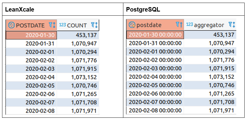
The results look fine in both databases. Let’s have a look at the query times:

We can find here the same issue with PostgreSQL as found with the ID aggregate; if we have a look at the average aggregate time value, we can see LeanXcale aggregating in 0.000032 ms/row, while Postgres aggregates in 0.00019 ms/row. Again, this is because, as LeanXcale inserts much faster, the aggregate that it must calculate aggregates many more rows than the aggregates PostgreSQL must calculate. Besides, the aggregate average time in LeanXcale is faster than the ID aggregate because there are fewer possible aggregate values, and thus, there are fewer rows to aggregate, and LeanXcale’s algorithm that pre-calculates the aggregation requires less effort to execute. So, we have Postgres loading 15 million rows in 4.21 hours and aggregating in 0.00019 ms/row; however, we have LeanXcale loading 15 million rows in 2.65 minutes and aggregating around 0.000032 ms/row.

SCENARIO 2: LX with delta tables versus PostgreSQL without a trigger structure

INSERTION TIME

Having just deleted the triggers and executing queries over Postgres with a usual count-group-by, let’s compare the insertion times again.

As a summary of the result times when inserting:

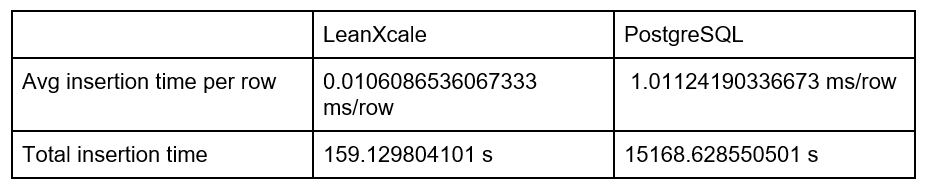
We can see here how Postgres gets better in insertion; this is normal because it doesn’t have to execute the trigger on each insertion. But LeanXcale still behaves much better in the insertion. In this scenario, we obtain a total insertion time gain of 98.70% with LeanXcale over PostgreSQL, and a row average insertion time gain of 98.70% with LeanXcale over PostgreSQL. In absolute value, and without triggers, PostgreSQL is storing 15 million rows in 3.37 hours, whereas LeanXcale does the same in 2.61 minutes.

QUERY EXECUTION

Now, let’s analyze the response times from the logs in this second scenario. These are the last 10 results for the first aggregator, based on our application’s cookie ID:

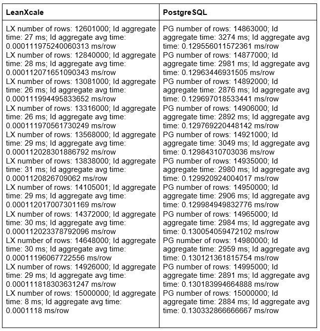
That’s the bad thing when using the count in PostgreSQL: the more rows a table has, the more time it takes to execute the count. LeanXcale is aggregating with an average time of 0.0001118 ms/row, while PostgreSQL is aggregating with an average time of 0.130332866666667 ms/row. This supposes a gain of 99.91% in average aggregation time with LeanXcale over PostreSQL. Please note the relative time, taking the insertion time into account: LeanXcale is inserting 15 million rows in 2.61 minutes and aggregating with an average time of 0.0001118 ms/row. PostgreSQL is inserting 15 million rows in 3.37 hours and aggregating with an average time of 0.130332866666667 ms/row.

About the date aggregator, the response times are:

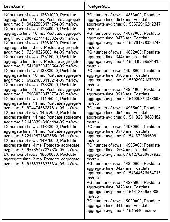
At this point, LeanXcale is aggregating with an average time of 0.0000319 ms/row, while PostgreSQL is aggregating with an average time of 0.1545946 ms/row. This supposes a gain of 99.97% in average aggregation time with LeanXcale over PostreSQL. Please note the relative time, taking the insertion time into account: LeanXcale is inserting 15 million rows in 2.61 minutes and aggregating with an average time of 0.0000319 ms/row. PostgreSQL is inserting 15 million rows in 3.37 hours and aggregating with an average time of 0.1545946 ms/row.

Conclusion

It is excellent to use deltas to obtain real-time metrics from data with very low execution times. It could be considered as a nice solution to one of the world’s database hotspots when performing analytical queries. Besides, and as usual for LeanXcale, it does not affect operational issues. So now, the use of pre-calculated aggregates at the time of insertion means a gain of about ~99% in insertion over PostgreSQL execution time, and a gain of about 66% or 99% in aggregation time, depending on the approach selected for aggregating in real-time with PostgreSQL. This is because getting the aggregate for a value simply requires reading a row from the relevant aggregate table, which is already pre-calculated, instead of doing a scan to find the right row and execute the aggregation or using heavy triggers to calculate it. LeanXcale seems to be the best fit for aggregating the number of cookies from users requesting to visit a web page in a hypothetical monitoring application. It is also the best for aggregating through dates and sessions of whatever register fields on the requests. Of course, this not only applies to our imaginary scenario but to any other we can imagine.

WRITTEN BY